| Tutorial deal.II 1 | Introductory example to illustrate the support for the finite elements method in DAE Tools (solution of a simple heat conduction equation). |
| Tutorial deal.II 2 | Solution of a simple transient heat convection-diffusion equation. |
| Tutorial deal.II 3 | Solution of the Cahn-Hilliard equation. |
| Tutorial deal.II 4 | Solution of a transient heat conduction using the various types of boundary conditions. |
| Tutorial deal.II 5 | Flow through porous media (Darcy’s law). |
| Tutorial deal.II 6 | A simple steady-state diffusion and first-order reaction in an irregular catalyst shape. |
| Tutorial deal.II 7 | Transient Stokes flow driven by the temperature differences in the fluid. |
| Tutorial deal.II 8 | Model of a small parallel-plate reactor with a catalytic surface (phenomena defined in two coupled FE systems with different dimensions: 2D and 1D). |
An introductory example of the support for Finite Elements in daetools. The basic idea is to use an external library to perform all low-level tasks such as management of mesh elements, degrees of freedom, matrix assembly, management of boundary conditions etc. deal.II library (www.dealii.org) is employed for these tasks. The mass and stiffness matrices and the load vector assembled in deal.II library are used to generate a set of algebraic/differential equations in the following form: [Mij]{dx/dt} + [Aij]{x} = {Fi}. Specification of additional equations such as surface/volume integrals are also available. The numerical solution of the resulting ODA/DAE system is performed in daetools together with the rest of the model equations.
The unique feature of this approach is a capability to use daetools variables to specify boundary conditions, time varying coefficients and non-linear terms, and evaluate quantities such as surface/volume integrals. This way, the finite element model is fully integrated with the rest of the model and multiple FE systems can be created and coupled together. In addition, non-linear and DAE finite element systems are automatically supported.
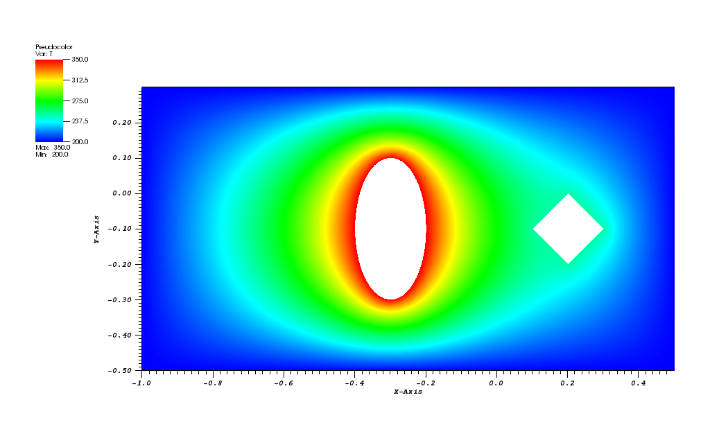
In this tutorial the simple transient heat conduction problem is solved using the finite element method:
dT/dt - kappa/(rho*cp)*nabla^2(T) = g(T) in Omega
The mesh is rectangular with two holes, similar to the mesh in step-49 deal.II example:
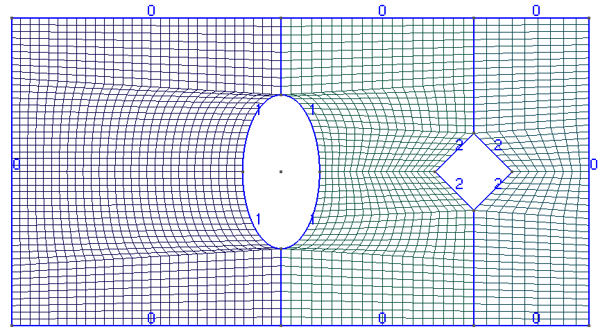
Dirichlet boundary conditions are set to 300 K on the outer rectangle, 350 K on the inner ellipse and 250 K on the inner diamond.
The temperature plot at t = 500s (generated in VisIt):
Animation:
Files
| Model report | tutorial_dealii_1.xml |
| Runtime model report | tutorial_dealii_1-rt.xml |
| Source code | tutorial_dealii_1.py |
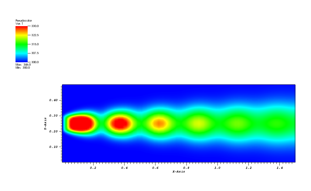
In this example a simple transient heat convection-diffusion equation is solved.
dT/dt - kappa/(rho*cp)*nabla^2(T) + nabla.(uT) = g(T) in Omega
The fluid flows from the left side to the right with constant velocity of 0.01 m/s. The inlet temperature for 0.2 <= y <= 0.3 is iven by the following expression:
T_left = T_base + T_offset*|sin(pi*t/25)| on dOmega
creating a bubble-like regions of higher temperature that flow towards the right end and slowly diffuse into the bulk flow of the fluid due to the heat conduction.
The mesh is rectangular with the refined elements close to the left/right ends:
-100x50.png)
The temperature plot at t = 500s:
Animation:
Files
| Model report | tutorial_dealii_2.xml |
| Runtime model report | tutorial_dealii_2-rt.xml |
| Source code | tutorial_dealii_2.py |
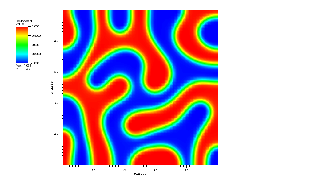
In this example the Cahn-Hilliard equation is solved using the finite element method. This equation describes the process of phase separation, where two components of a binary mixture separate and form domains pure in each component.
dc/dt - D*nabla^2(mu) = 0, in Omega
mu = c^3 - c - gamma*nabla^2(c)
The mesh is a simple square (0-100)x(0-100):

The concentration plot at t = 500s:
Animation:
Files
| Model report | tutorial_dealii_3.xml |
| Runtime model report | tutorial_dealii_3-rt.xml |
| Source code | tutorial_dealii_3.py |
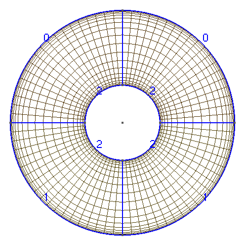
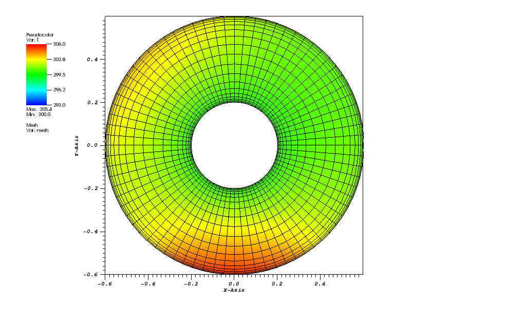
In this tutorial the transient heat conduction problem is solved using the finite element method:
dT/dt - kappa * nabla^2(Τ) = g in Omega
The mesh is a pipe submerged into water receiving the heat of the sun at the 45 degrees from the top-left direction, the heat from the suroundings and having the constant temperature of the inner tube. The boundary conditions are thus:
The pipe mesh is given below:
The temperature plot at t = 3600s:
Animation:
Files
| Model report | tutorial_dealii_4.xml |
| Runtime model report | tutorial_dealii_4-rt.xml |
| Source code | tutorial_dealii_4.py |
In this example a simple flow through porous media is solved (deal.II step-20).
K^{-1} u + nabla(p) = 0 in Omega
-div(u) = -f in Omega
p = g on dOmega
The mesh is a simple square:
x(-1,1)-50x50.png)
The velocity magnitude plot:
Files
| Model report | tutorial_dealii_5.xml |
| Runtime model report | tutorial_dealii_5-rt.xml |
| Source code | tutorial_dealii_5.py |
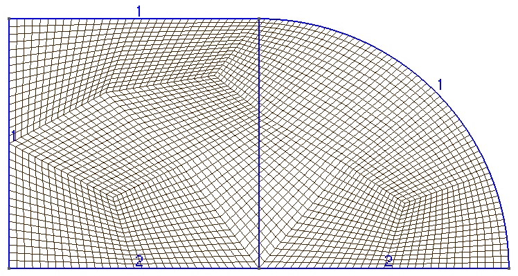
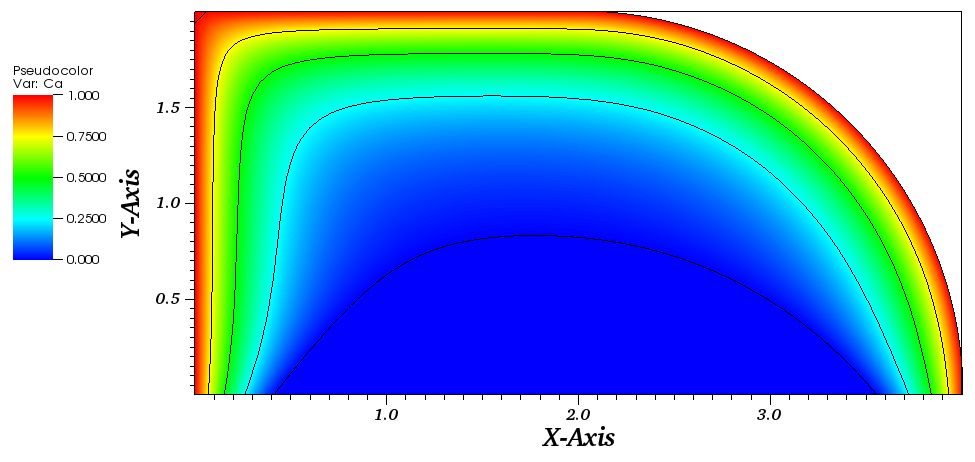
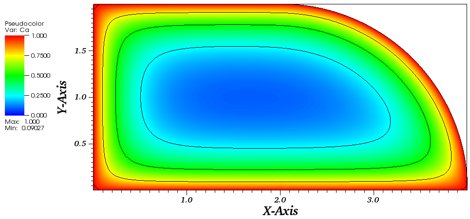
A simple steady-state diffusion and first-order reaction in an irregular catalyst shape (Proc. 6th Int. Conf. on Mathematical Modelling, Math. Comput. Modelling, Vol. 11, 375-319, 1988) applying Dirichlet and Robin type of boundary conditions.
D_eA * nabla^2(C_A) - k_r * C_A = 0 in Omega
D_eA * nabla(C_A) = k_m * (C_A - C_Ab) on dOmega1
C_A = C_Ab on dOmega2
The catalyst pellet mesh:
The concentration plot:
The concentration plot for Ca=Cab on all boundaries:
Files
| Model report | tutorial_dealii_6.xml |
| Runtime model report | tutorial_dealii_6-rt.xml |
| Source code | tutorial_dealii_6.py |
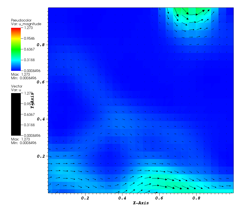
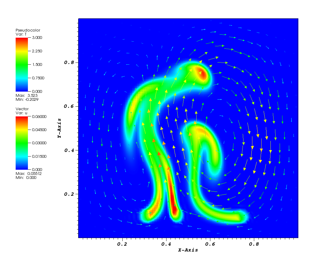
In this example 2D transient Stokes flow driven by the differences in buoyancy caused by the temperature differences in the fluid is solved (deal.II step-31).
The differences to the original problem are that the grid is not adaptive and no stabilisation method is used.
The problem can be described using the Stokes equations:
-div(2 * eta * eps(u)) + nabla(p) = -rho * beta * g * T in Omega
-div(u) = 0 in Omega
dT/dt + div(u * T) - div(k * nabla(T)) = gamma in Omega
The mesh is a simple square (0,1)x(0,1):
x(0,1)-50x50.png)
The temperature and the velocity vectors plot:
Animation:
Files
| Model report | tutorial_dealii_7.xml |
| Runtime model report | tutorial_dealii_7-rt.xml |
| Source code | tutorial_dealii_7.py |
In this example a small parallel-plate reactor with an active surface is modelled.
This problem and its solution in COMSOL Multiphysics software is described in the Application Gallery: Transport and Adsorption (id=5).
The transport in the bulk of the reactor is described by a convection-diffusion equation:
dc/dt - D*nabla^2(c) + div(uc) = 0 in Omega
The material balance for the surface, including surface diffusion and the reaction rate is:
dc_s/dt - Ds*nabla^2(c_s) = -k_ads * c * (Gamma_s - c_s) + k_des * c_s in Omega_s
For the bulk, the boundary condition at the active surface couples the rate of the reaction at the surface with the flux of the reacting species and the concentration of the adsorbed species and bulk species:
n⋅(-D*nabla(c) + c*u) = -k_ads*c*(Gamma_s - c_s) + k_des*c_s
The boundary conditions for the surface species are insulating conditions.
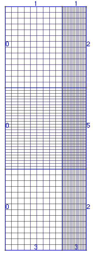
The problem is modelled using two coupled Finite Element systems: 2D for bulk flow and 1D for the active surface. The linear interpolation is used to determine the bulk flow and active surface concentrations at the interface.
The mesh is rectangular with the refined elements close to the left/right ends:
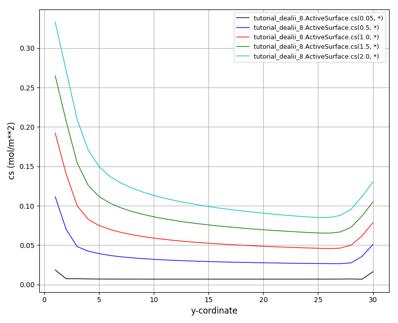
The cs plot at t = 2s:
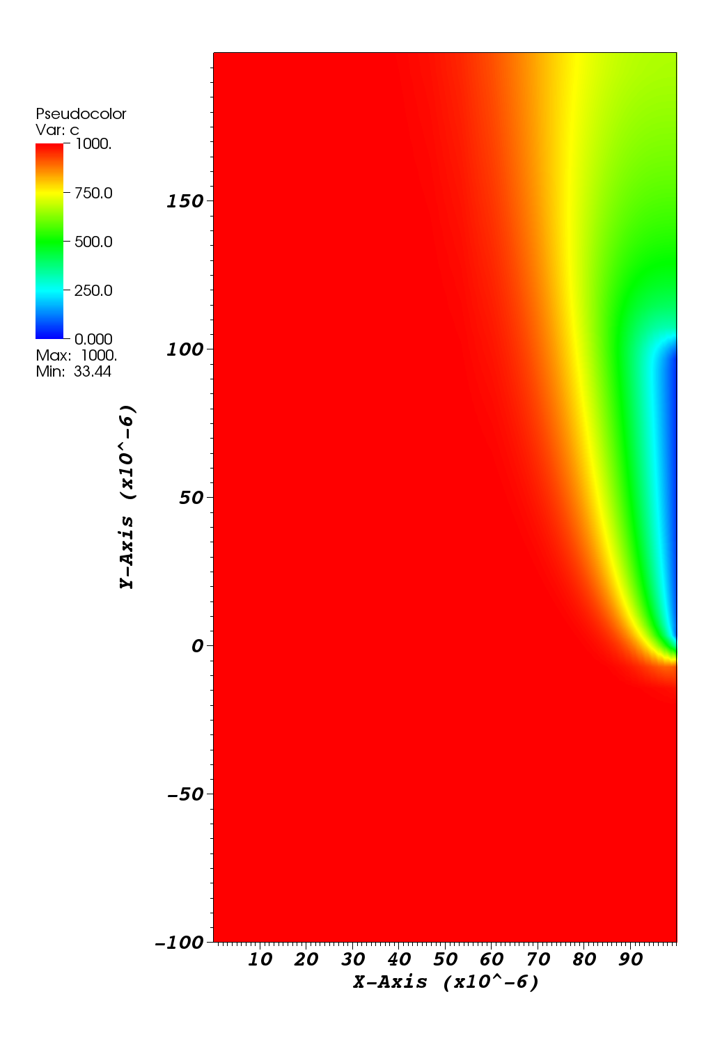
The c plot at t = 2s:
Animation:
Files
| Model report | tutorial_dealii_8.xml |
| Runtime model report | tutorial_dealii_8-rt.xml |
| Source code | tutorial_dealii_8.py |